It is quite common to hear complaints about the steep learning curve of R. And it is true that it would take time to grasp its versatility (if it is possible at all). Nevertheless, there are many packages that give the opportunity of experiencing the power of R for beginners. One notable example is Zelig package (Choirat et al. 2017). The online documentation provides examples for a wide range of models. As one can see in these examples, Zelig favors the use of simulation-based approach in estimating, interpreting, and presenting results of statistical analysis. King, Tomz, and Wittenberg (2000, 348) listed three advantages of this approach:

First, and most importantly, it can extract new quantities of interest from standard statistical models, thereby enriching the substance of social science research. Second, our approach allows scholars to assess the uncertainty surrounding any quantity of interest, so it should improve the candor and realism of statistical discourse about politics. Finally, our method can convert raw statistical results into results that everyone, regardless of statistical training, can comprehend.

Of course, easy-to-use does not necessarily mean easy to interpret and present: “researchers who put [these methods] into practice will have to think much harder about which quantities are of interest and how to communicate to a wider audience” (King, Tomz, and Wittenberg 2000, 360). Lets see an example using well-known Mroz’ data:

library(Zelig)
library(texreg) #for html table
df <- carData::Mroz
logit_zelig <- zelig(lfp ~ k5 + k618 + age + wc + hc + lwg, 
                     data=df, model = "logit", cite=FALSE)
summary(logit_zelig, odds_ratio=TRUE)

## Model: 
## 
## Call:
## stats::glm(formula = lfp ~ k5 + k618 + age + wc + hc + lwg, family = binomial("logit"), 
##     data = as.data.frame(.))
## 
## Deviance Residuals: 
##     Min       1Q   Median       3Q      Max  
## -2.0875  -1.1168   0.6377   0.9797   2.1894  
## 
## Coefficients:
##             Estimate (OR) Std. Error (OR) z value Pr(>|z|)    
## (Intercept)      18.88881        11.87495   4.674 2.95e-06 ***
## k5                0.23725         0.04590  -7.436 1.03e-13 ***
## k618              0.91635         0.06119  -1.308 0.190810    
## age               0.93358         0.01168  -5.492 3.98e-08 ***
## wcyes             1.99876         0.44711   3.096 0.001962 ** 
## hcyes             0.86741         0.16830  -0.733 0.463476    
## lwg               1.75248         0.26083   3.769 0.000164 ***
## ---
## Signif. codes:  0 '***' 0.001 '**' 0.01 '*' 0.05 '.' 0.1 ' ' 1
## 
## (Dispersion parameter for binomial family taken to be 1)
## 
##     Null deviance: 1029.75  on 752  degrees of freedom
## Residual deviance:  924.77  on 746  degrees of freedom
## AIC: 938.77
## 
## Number of Fisher Scoring iterations: 4

As we can see in the output, zelig function calls glm from stats. The following steps, however, illustrate how simulation approach is used to estimate expected and predicted values.

x_no_college <- setx(logit_zelig, wc = "no")
x_college <- setx1(logit_zelig, wc = "yes")
sim_logit_zelig <- sim(logit_zelig, x = x_no_college, x1 = x_college)
summary(sim_logit_zelig)

## 
##  sim x :
##  -----
## ev
##           mean         sd       50%      2.5%     97.5%
## [1,] 0.5434036 0.02483741 0.5435714 0.4962461 0.5904441
## pv
##         0    1
## [1,] 0.46 0.54
## 
##  sim x1 :
##  -----
## ev
##           mean         sd       50%      2.5%     97.5%
## [1,] 0.7008201 0.04802893 0.7038947 0.6022215 0.7840549
## pv
##          0     1
## [1,] 0.277 0.723
## fd
##           mean         sd       50%       2.5%     97.5%
## [1,] 0.1574164 0.04701865 0.1604971 0.06458937 0.2430327

Now, we might want to estimate predicted probabilities over the range of a predictor for both levels of wc.

logit_zelig <- zelig(lfp ~ k5 + k618 + age + wc + hc + lwg, 
                     data=df, model = "logit", cite=FALSE)

x_no_college  <- setx(logit_zelig, wc = "no",  age = 30:60)
x_college <- setx(logit_zelig, wc = "yes",  age = 30:60)
sim_logit_zelig <- sim(logit_zelig, x = x_no_college, x1 = x_college)
ci.plot(sim_logit_zelig, ylab = "Predicted Probability of Labor Force Participation")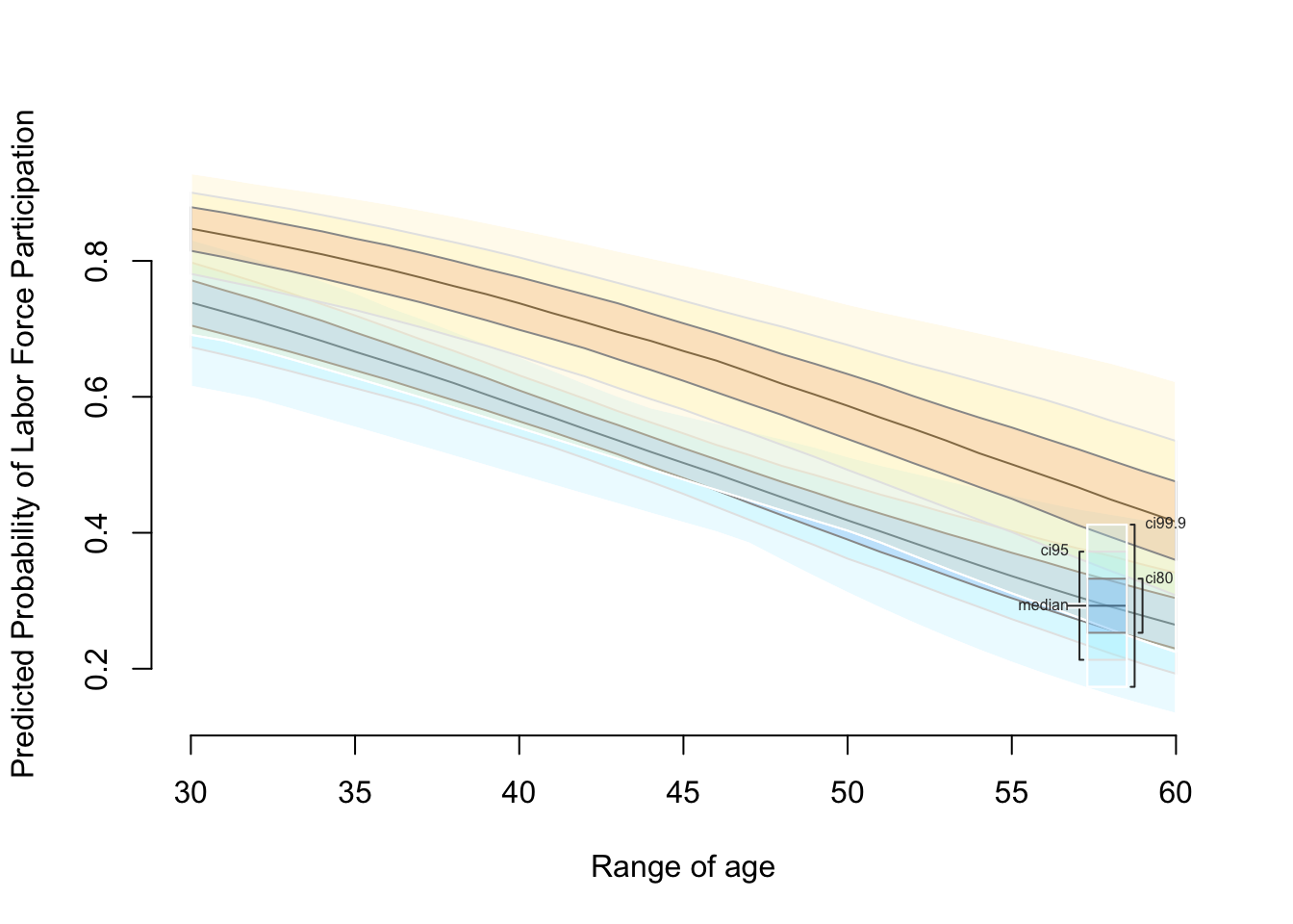

Another nice feature of Zelig package is the exterior interaction functions which help to extract information from Zelig object. For example, from_zelig_model() makes it easy to extract model results and pass them into a table function.

df_logit_model <- from_zelig_model(logit_zelig)
htmlreg(df_logit_model, center=FALSE, caption = " ")

Actually, texreg functions accept zelig class objects:

logit_zelig1 <- zelig(lfp ~ k5 + age, 
                      data=df, model = "logit", cite=FALSE)
logit_zelig2 <- zelig(lfp ~ k5 + age + wc, 
                      data=df, model = "logit", cite=FALSE)
logit_zelig3 <- zelig(lfp ~ k5 + age + wc + lwg, 
                      data=df, model = "logit", cite=FALSE)
logit_zelig4 <- zelig(lfp ~ k5 + age + wc + lwg + inc, 
                      data=df, model = "logit", cite=FALSE)
htmlreg(list(logit_zelig1, logit_zelig2, logit_zelig3, logit_zelig4), 
        center=FALSE, caption = " ")

<!DOCTYPE HTML PUBLIC “-//W3C//DTD HTML 4.01 Transitional//EN” “http://www.w3.org/TR/html4/loose.dtd”>

	Model 1	Model 2	Model 3	Model 4
(Intercept)	3.09***	2.92***	2.44***	2.90***
	(0.50)	(0.50)	(0.52)	(0.54)
k5	-1.32***	-1.41***	-1.41***	-1.43***
	(0.19)	(0.19)	(0.19)	(0.19)
age	-0.06***	-0.06***	-0.06***	-0.06***
	(0.01)	(0.01)	(0.01)	(0.01)
wcyes		0.83***	0.62**	0.87***
		(0.18)	(0.19)	(0.21)
lwg			0.57***	0.62***
			(0.15)	(0.15)
inc				-0.03***
				(0.01)
AIC	970.48	950.86	937.09	918.46
BIC	984.36	969.36	960.21	946.20
Log Likelihood	-482.24	-471.43	-463.54	-453.23
Deviance	964.48	942.86	927.09	906.46
Num. obs.	753	753	753	753
p < 0.001, p < 0.01, p < 0.05

References

Choirat, Christine, James Honaker, Kosuke Imai, Gary King, and Olivia Lau. 2017. Zelig: Everyone’s Statistical Software. http://zeligproject.org/.
Imai, Kosuke, Gary King, and Olivia Lau. 2008. “Toward a Common Framework for Statistical Analysis and Development.” Journal of Computational Graphics and Statistics 17 (4): 892–913. http://j.mp/msE15c.
King, Gary, Michael Tomz, and Jason Wittenberg. 2000. “Making the most of statistical analyses: Improving interpretation and presentation.” American Journal of Political Science 44 (13-2): 341–55.
Leifeld, Philip. 2013. “texreg: Conversion of Statistical Model Output in R to LaTeX and HTML Tables.” Journal of Statistical Software 55 (8): 1–24. http://www.jstatsoft.org/v55/i08/.